Build visually.
Place and adjust peaks on the plot. Add backgrounds and custom functions, and inspect each component.
 CurveMole
FREE, OPEN-SOURCE SCIENTIFIC SOFTWARE
Extensible scientific analysis.
Build models visually, analyse individual curves or full series, and inspect residuals and parameter uncertainty in one modular desktop toolbox.
Spectroscopy · Diffraction · Kinetics · Experimental x–y data
Explore the workflow ↓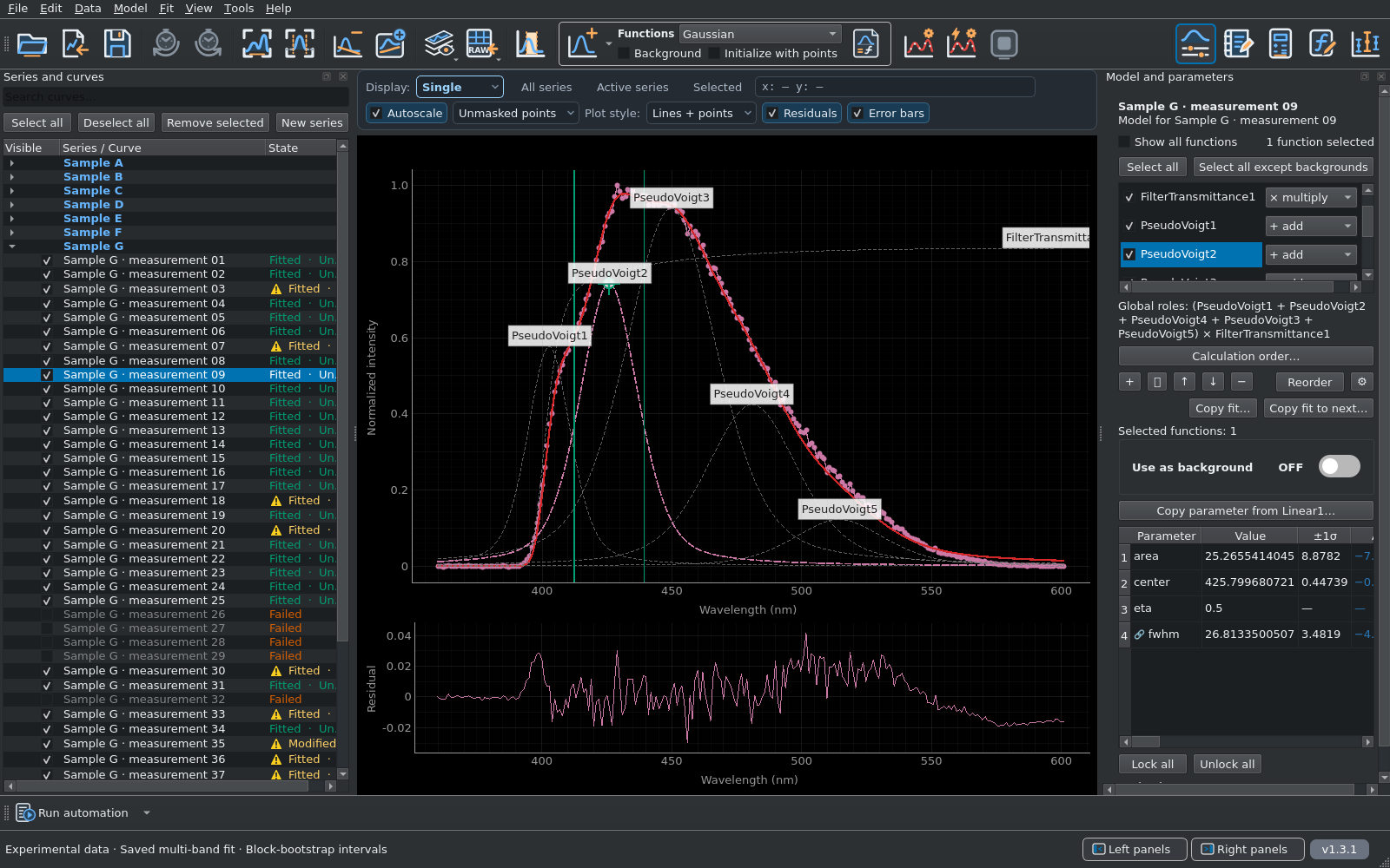
Measured fluorescence data: five pseudo-Voigt profiles multiplied by filter transmittance. The saved project contains 14 series and 98 curves, with block-bootstrap intervals, residual structure and attention flags retained. Sample and measurement labels have been renamed. Project provenance ↗
Import → Build a model → Fit → Inspect → Save and export
Place and adjust peaks on the plot. Add backgrounds and custom functions, and inspect each component.
Set bounds, fix values and define relationships within a curve or across several datasets.
Apply reversible masks and transformations while retaining your imported data.
Keep models, results and laboratory notes in a portable project. Export data, parameters, figures and reports together.
Follow changes with temperature, pressure or time.
Compare the data, then choose how to fit the series.
Analyse individual datasets with their own models and parameters.
Carry a prepared model through the series, with inspection and pause/resume.
Fit several curves in one optimisation, linking shared or related quantities.
Use vertical offsets to compare peak positions, widths and amplitudes across related curves.
View documentation ↗Illustrative Raman-like data. Actual application screenshots.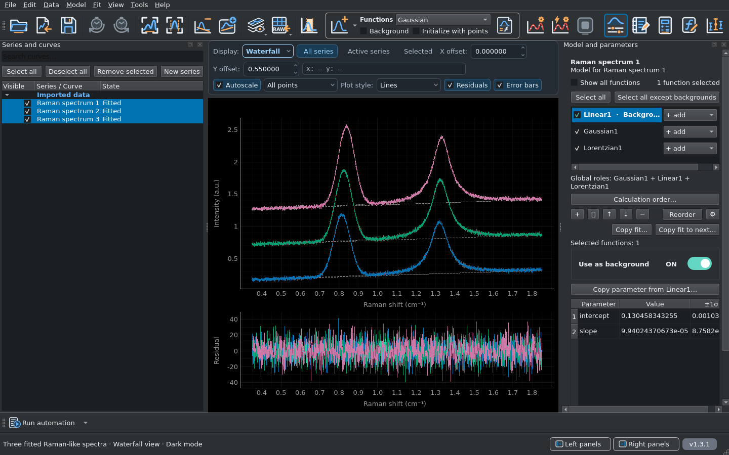
Examine residual structure, parameter correlations and confidence intervals. Choose additional uncertainty analyses to suit your model and noise assumptions.
Uncertainty methods and assumptions ↗For weighted least squares with supplied standard deviations in y, the objective is
Here θ denotes the free model parameters. X uncertainties and correlations between data points are not included in this objective.
Weighting conventions ↗Start with the graphical interface, without writing code.
Add custom models and procedures when you need them.
Define analytical expressions and reuse your model functions across analyses.
Define a custom function ↗Install community extensions for additional analyses, fitting algorithms and exporters. Browse the catalog from File → Plugin Manager.
Browse community plugins ↗Create or share a plugin ↗Automate import, preprocessing, fitting and export, or integrate CurveMole with other software.
Python API ↗YAML workflows ↗AI-assisted automation. Give an AI assistant the Python API audit or YAML workflow audit to help write scripts and workflows. These self-contained interface references avoid loading the entire codebase into the AI’s context, saving tokens. Use the audit matching your installed version, and review the scientific assumptions.
One scientific engine, shared by the desktop interface, Python API, command line and YAML workflows.
Inspect fitted models and residuals, download the projects, or compare the interface themes.
Three reproducible examples of weighted nonlinear least squares.
Data, fitted models and normalized residuals are shown together.
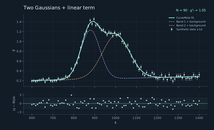
Two Gaussian components and a linear term fitted simultaneously to data with nonuniform uncertainties. Individual components are displayed with the linear term added.
y(x) = b₀ + b₁x + G₁(x) + G₂(x)The fit reports strong parameter correlation (|r| ≥ 0.95), illustrating why residuals and parameter covariance should be examined together.
Fit: CurveMole · Plot: Matplotlib
Website styling; not an application screenshot.
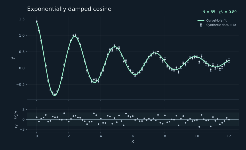
A user-defined function combines amplitude, frequency, phase, exponential damping and an offset. All five parameters are estimated in one weighted fit.
y(x) = c + A exp(−x/τ) cos(ωx + φ)A general x–y analysis example: the model is entered as a custom formula using the same engine as the desktop interface.
Fit: CurveMole · Plot: Matplotlib
Website styling; not an application screenshot.
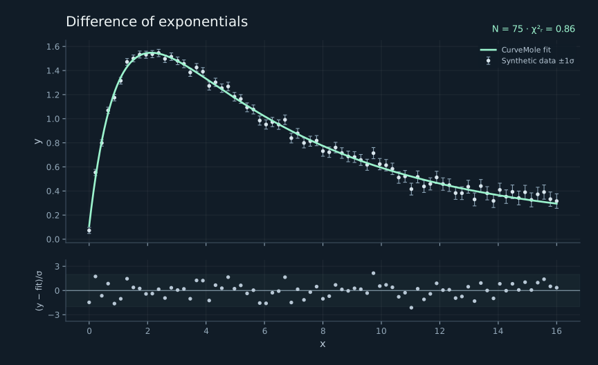
A custom formula combines two exponential terms. The amplitude, offset and two exponential coefficients are refined with explicit parameter bounds.
y(x) = c + A [exp(−k₁x) − exp(−k₂x)]Nonuniform uncertainties enter the fitting objective explicitly. Bounds separate the two exponential coefficients.
Fit: CurveMole · Plot: Matplotlib
Website styling; not an application screenshot.
Fitting engine: CurveMole 0.46.0 · Figure rendering: Matplotlib with a website-specific style · fixed random seed · supplied σ treated as absolute · parameter uncertainties from local covariance. These examples demonstrate the workflow; they are not experimental validation of the software. Reproduce the examples ↓
The same illustrative Raman dataset in both display modes.
Drag the divider to compare the interface.
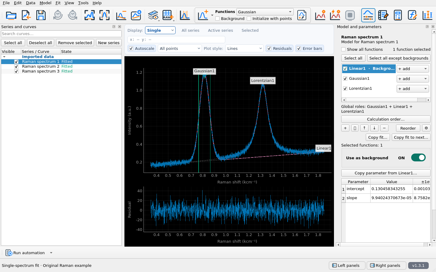
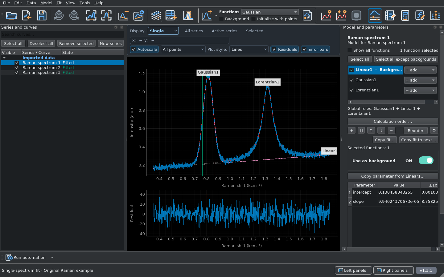
Illustrative Raman-like data · Matched viewport and model · Actual application screenshots
Download CurveMole, import a curve and build your first model.
The quick start walks you through fitting, inspection and export.