 CurveMole
One isolated band. Two overlapping bands.
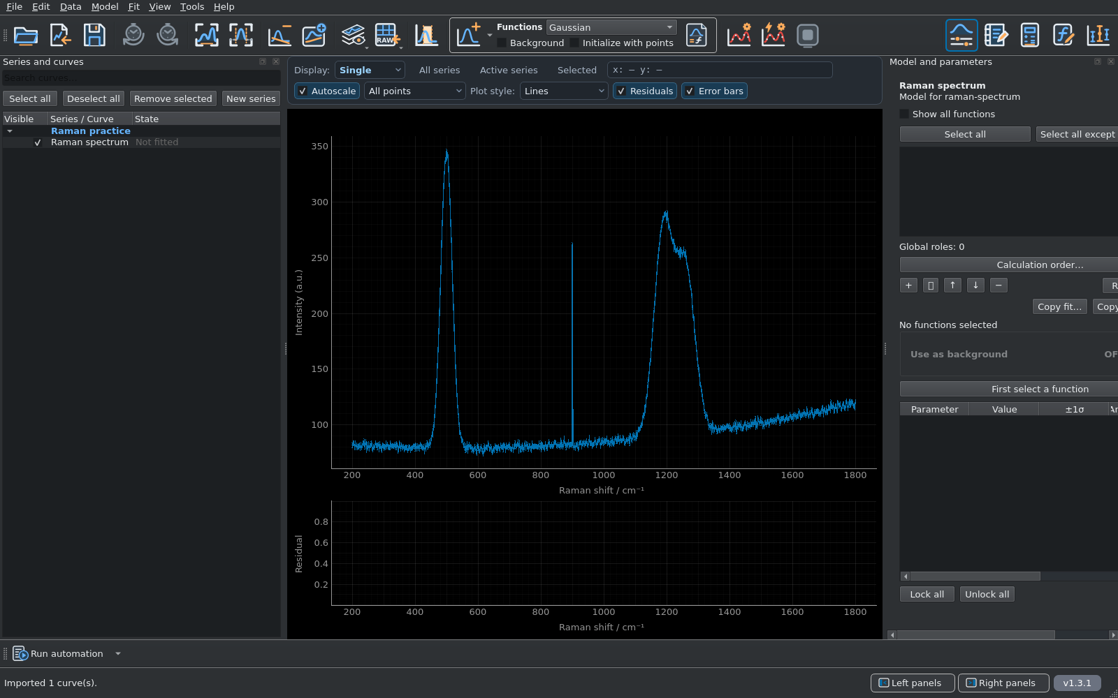
The input contains 801 samples from 200 to 1800 cm−1, three Gaussian bands, a quadratic background and independent Gaussian noise with known standard deviation σy = 2. A narrow positive artefact at 900 cm−1 lets you practise masking.
Unzip the practice pack into a working folder. Keep the original CSV files and use a separate folder for your exports. All data are simulated; Gaussian profiles are chosen for this exercise.
Click any screenshot to inspect the full-size image. The screenshot set and its version record are regenerated from the selected stable CurveMole build when the website is published.
Load the spectrum and its Y errors.
- Open CurveMole and choose File → Import data… (Ctrl+I). Select
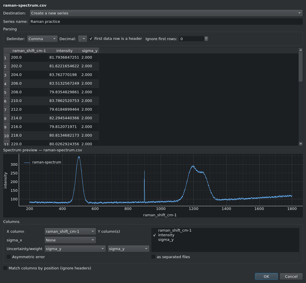
raman-spectrum.csv. - In the import mapping, choose raman_shift_cm-1 for X and intensity for Y.
- Map the third column, sigma_y, as a symmetric standard deviation: choose sigma_y under Uncertainty/weight and select the sigma_y column. It is a one-standard-deviation error, not a 95% interval.
- Check the preview, confirm the import and activate the curve in Series and curves.
Exclude the artefact from the fit.
- Click the graphical Mask button.
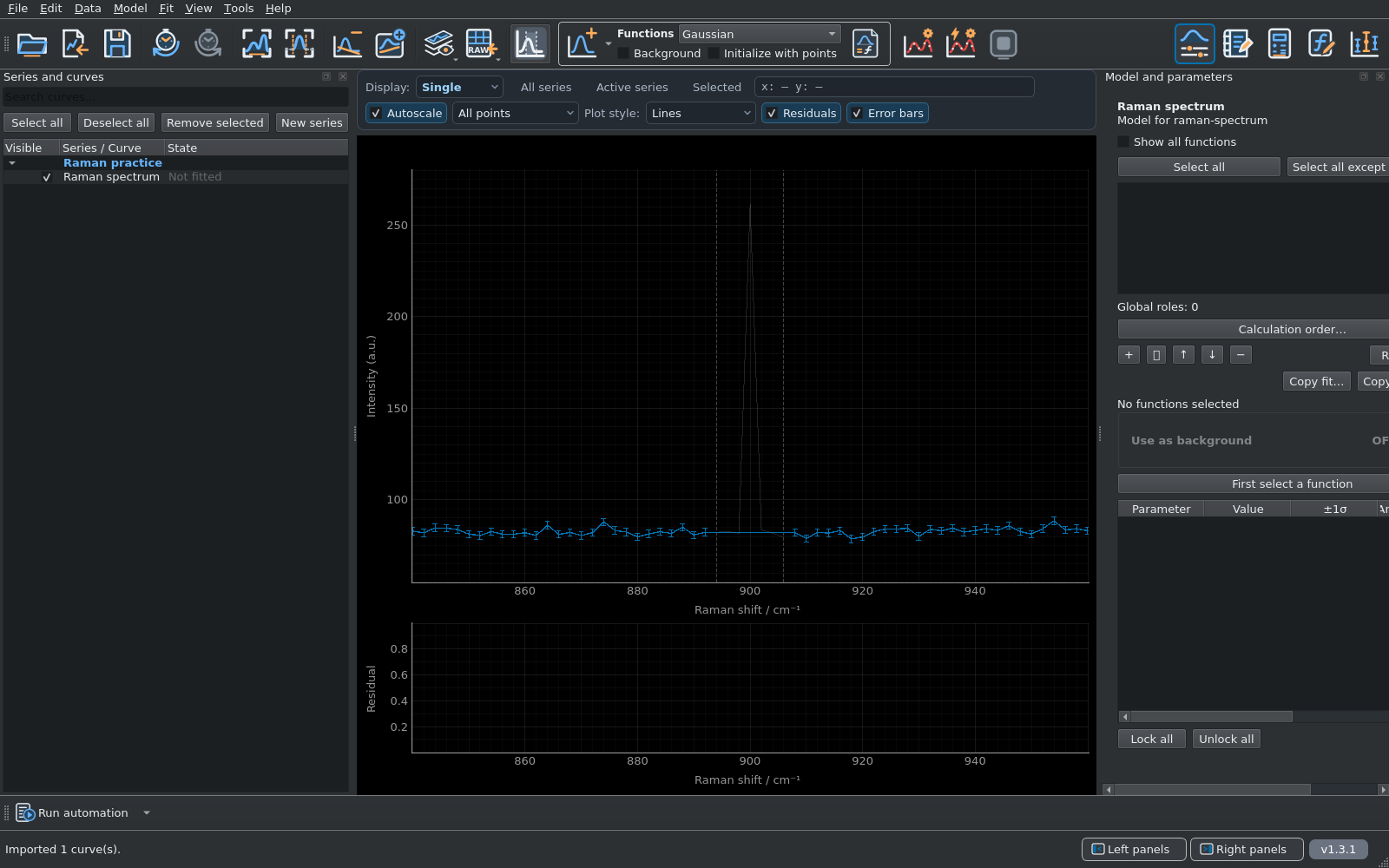
- Right-drag over approximately 894–906 cm−1, covering the spike. The reference analysis excludes seven sampled points in this interval.
- Check the shaded interval and faded points. Click Mask again to return to normal graph navigation. Left-drag in mask mode removes a mask; Undo also reverses it.
Masking changes which observations enter the fit. It leaves their measured values intact. In this simulated example the artefact is known; a narrow feature in real data needs a scientific reason for exclusion.
Create a quadratic background from three points.
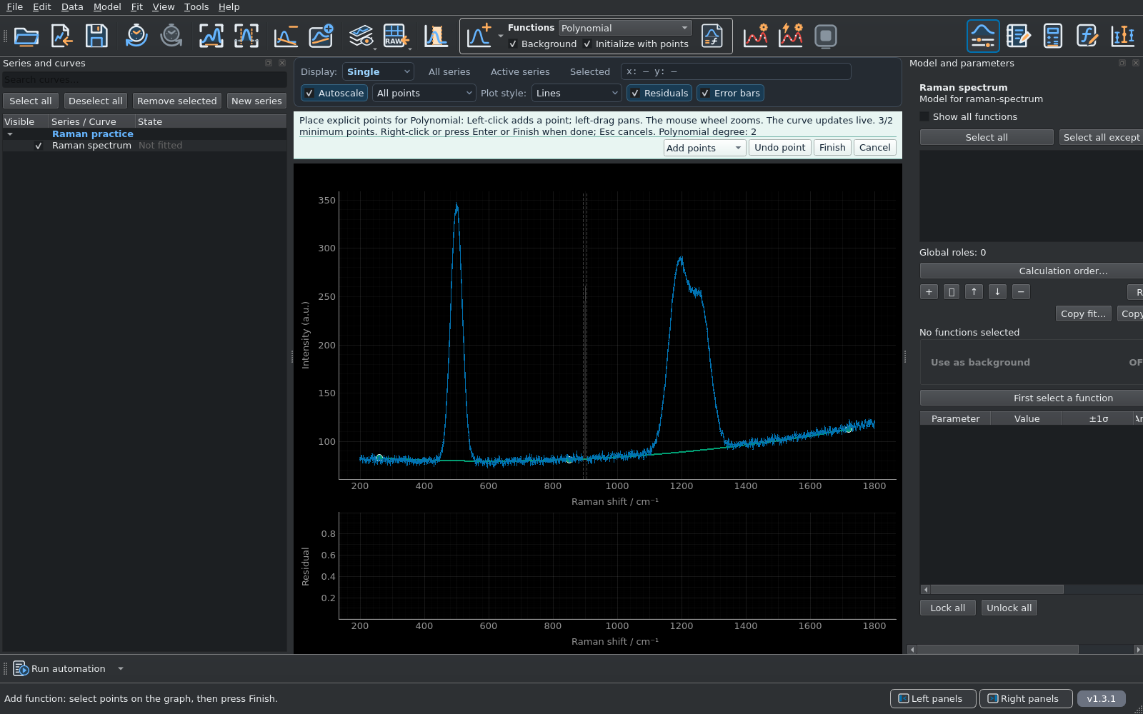
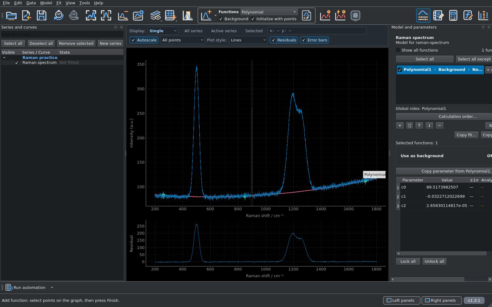
- Choose Polynomial in the function selector. Enable Initialize with points and Background, then press Add.
- Place three points in the peak-free regions listed below. Use the observed intensity near each coordinate; the green preview shows the polynomial being constructed.
- Use Move points, Delete points or Undo point if needed. Press Finish after the third point.
- Check Polynomial in Model and parameters: it has c0, c1 and c2, is marked as background and its point-initialised parameters are fixed.
| Raman shift / cm−1 | Observed intensity / a.u. |
|---|---|
| 260 | 82.924 |
| 850 | 81.293 |
| 1720 | 112.654 |
Three points means degree 2. Polynomial degree follows the number of distinct control points minus one. A fourth point creates a cubic polynomial; it does not add another observation to a quadratic fit. These points initialise the background function rather than fitting it to every measured point.
Subtract the polynomial from the data.
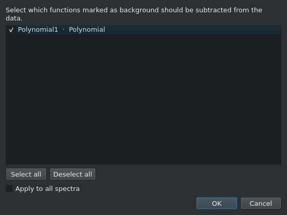
- Choose Data → Subtract background….
- Keep the polynomial selected in the background list and confirm with OK.
- Inspect the corrected spectrum. CurveMole records the subtraction and disables the polynomial component so it will not be counted again in the next fit.
This operation changes the data supplied to subsequent fits while preserving the imported originals. The display-only command Remove fitted background in this view is a different operation and is not used here.
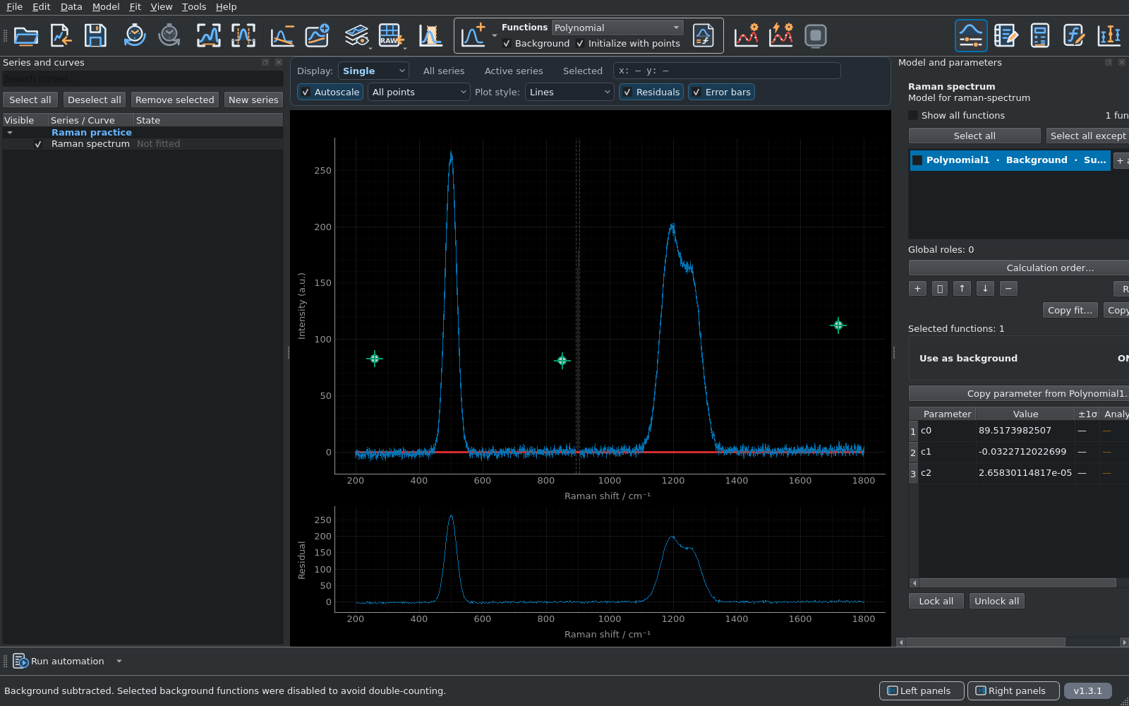
Your clicked points may differ slightly from the reference coordinates. Small differences in the fitted parameters are therefore expected. The exact chosen polynomial is included in background-reference.csv.
Place three Gaussian bands.
- Choose Gaussian, clear Background and keep Initialize with points enabled.
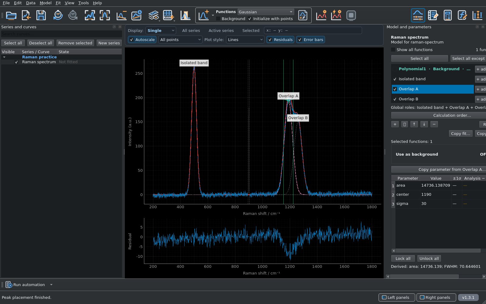
- Press Add. Click a band centre and drag horizontally to a half-height edge to set its initial width. Place one isolated band and the two overlapping contributions, then press Finish.
- Use the approximate positions and widths below as starting estimates. The overlap makes individual heights difficult to read; the fit will refine the parameters.
- To match the reference labels, right-click each function and choose Rename function…: use Isolated band, Overlap A and Overlap B.
- Select each Gaussian in turn. In its parameter table set the Lower bound for area to 0, appropriate for these simulated positive bands. Leave the band parameters free; keep their Fixed boxes clear.
| Function | Centre / cm−1 | Initial FWHM / cm−1 | Gaussian σ / cm−1 |
|---|---|---|---|
| Isolated band | 500 | ≈42 | ≈18 |
| Overlap A | 1190 | ≈71 | ≈30 |
| Overlap B | 1260 | ≈71 | ≈30 |
Gaussian parameters are area, center and sigma; area is integrated intensity, not peak height. Keep the band parameters free and the polynomial disabled. Widths must remain positive.
Run and inspect the first fit.
- Keep the tutorial spectrum active, with no other curves selected.
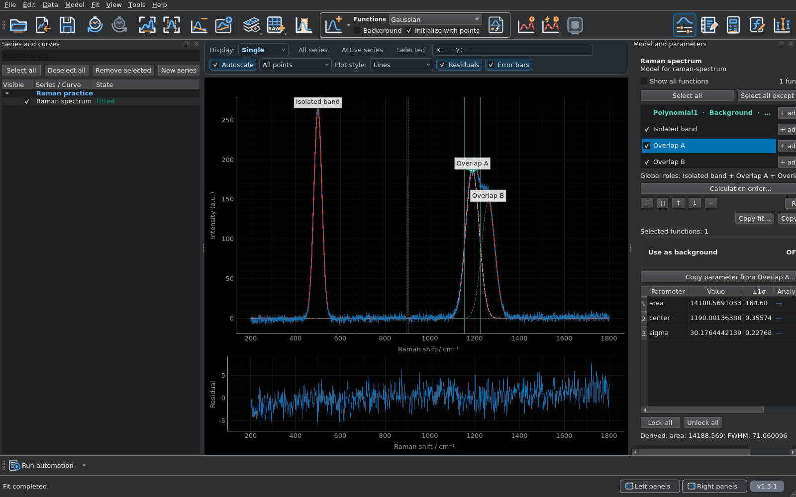
- Click Quick Fit. On first use it runs an independent local least-squares fit with the default linear loss and the imported σy values enabled as data errors.
- Wait for the spectrum to be marked Fitted, then inspect the total fit, each band and the residual panel.
The reference fit uses 794 unmasked observations and nine free Gaussian parameters. Supplied σy values are treated as absolute noise scales. Check convergence and residual structure before interpreting the parameter errors.
Inspect the covariance intervals.
- Choose Fit → Uncertainty Analysis.
- Select Fit covariance and Active spectrum, then press Run explicit uncertainty analysis. This displays the local covariance estimate already available from the fit.
- Read the fitted value and lower/upper confidence limits for each free parameter. Keep the original ±1σ fit errors distinct from later explicit-analysis intervals.
These confidence intervals use a local covariance approximation around the fitted solution. The next step uses Monte Carlo samples to examine uncertainty and the coupling between overlapping-band areas.
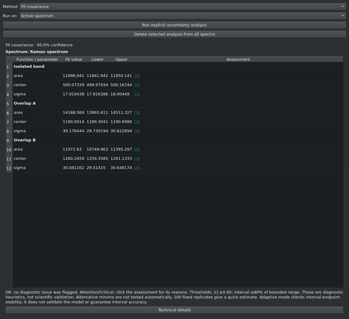
The polynomial background was estimated from three observed points, held fixed and subtracted. Its estimation uncertainty is not propagated into these band intervals. The reported errors are conditional on that chosen background.
Resample and inspect the overlapping bands.
- In the same panel, select Parametric Monte Carlo and Active spectrum.
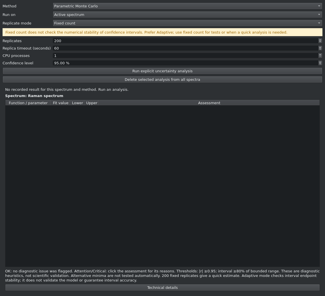
- For this short exercise choose Fixed count, 200 replicates and 95% confidence. Set CPU processes to 1 to match this reference run, and leave the per-replica timeout at its default.
- Press Run explicit uncertainty analysis. CurveMole generates data from the fitted model and the imported noise scale, then refits each replica.
- Inspect the completed/failed counts, interval bounds and assessment reasons. Select the displayed uncertainty method in the model panel if you want the Monte Carlo minus/plus errors shown beside each fitted value.
- With Parametric Monte Carlo still selected, find the area row for Overlap A. Click its Attention assessment to read the correlation with Overlap B area.
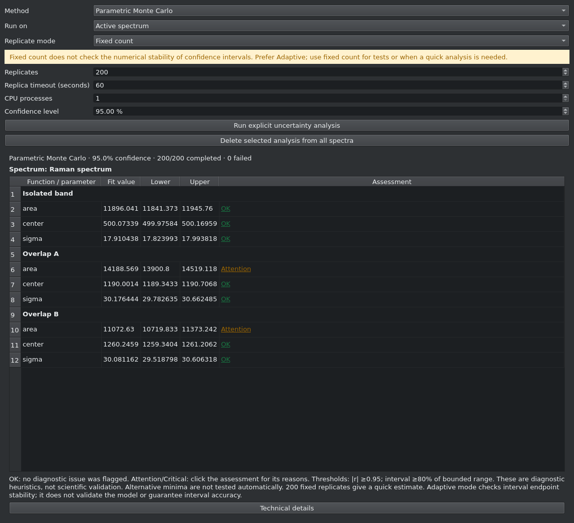
The reference Monte Carlo samples show a strong negative area correlation: r ≈ −0.97. One overlapping area can increase while the other decreases, with relatively little change in their sum. This is an empirical correlation across the refitted replicas; the local covariance of the original fit gives a separate estimate, r ≈ −0.97.
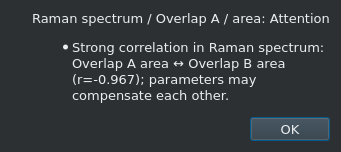
This is a correlation between parameter estimates in the chosen model. It does not by itself establish a physical relationship between the Raman bands.
200 fixed replicates illustrate the procedure; they do not establish interval stability. For intervals you intend to report, prefer Adaptive - stop when intervals stabilize and inspect its stopping reason and failed fits. In both covariance and Monte Carlo here, the estimated, subtracted background is held fixed: its uncertainty is not propagated into the band parameters.
Export the observations and fitted traces.
- Choose File → Quick export: spectra and fit curves… (Ctrl+T), select this spectrum and choose an output folder.
- Include Individual fit functions/components, Total fit and Residuals (data - total fit).
- Leave Export spectrum with fitted background subtracted unchecked: the processing step already subtracted our polynomial.
- For the complete 801-row record, leave Export only non-masked points unchecked. For a separate table containing only the 794 fitted observations, export again with that option checked.
- Confirm. CurveMole writes one multi-column file named from the source spectrum, with descriptive headers for the observations and selected traces.
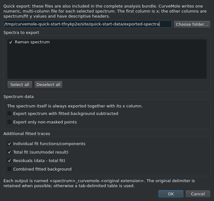
If you include Combined fitted background, its column is zero in this model because the subtracted polynomial is disabled. It does not recover the original baseline; the reference exports leave this option unchecked. Keep the raw CSV and the supplied chosen-background table when reconstructing the whole processing sequence.
The reference downloads use the shorter names fit-curves.csv and fit-curves-unmasked.csv. To reproduce the plot outside CurveMole, keep replot.py, fit-curves.csv and background-reference.csv in one folder. With pandas and Matplotlib installed, run python replot.py there. It writes replotted-fit.png with the data, components, total fit and residuals; excluded points remain identified.
Export every function parameter.
- Choose File → Quick export: function parameters… and save the CSV in your results folder.
- Check Also export covariance matrices if you want the labelled fit covariance and, when available, a separate covariance from the selected Monte Carlo samples.
- Open the table in a spreadsheet or analysis program. The first two header rows identify the functions and their parameters; each spectrum occupies one data row.
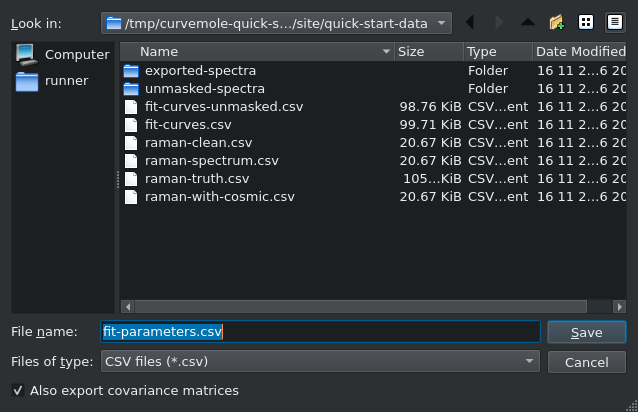
The table contains Gaussian area, center and sigma values and their errors, plus the polynomial coefficients retained in the project. Fixed background coefficients have no fitted uncertainty. The original fit-error columns and the selected explicit-analysis error columns describe different estimates.
Keep the project and the full analysis bundle.
- Choose File → Save project and save a .fitproj file. It retains original data, the mask, the subtraction, models and recorded analyses.
- Choose File → Export analysis bundle… (Ctrl+E). Select the numeric spectra, function parameters, uncertainty intervals/matrices, figures and a portable project copy.
- Export into a named results folder. Start with its README.txt to find the data tables, figures, reports and saved project.
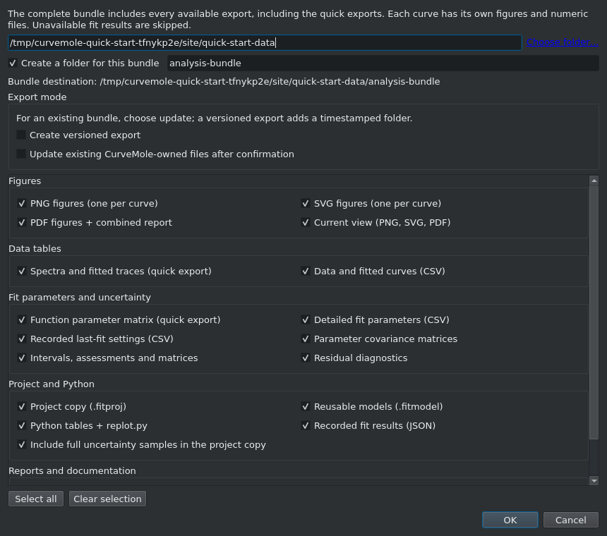
Keep the software version, model, weighting and uncertainty method with the results. The practice pack includes the completed reference project so you can inspect the recorded state or compare it with your own.
Load and use the cosmic-ray removal plugin.
Do this on a fresh copy of the raw spectrum after saving your fitted project. The optional exercise demonstrates an alternative treatment of the same injected artefact.
- Download the cosmic-ray removal plugin and extract it. Keep the manifest and Python module together in the
cosmic_ray_removalfolder. - Choose File → New project and import
raman-with-cosmic.csv, using the same X/Y/σy mapping as step 1. Leave this copy unmasked and without background subtraction. - Open File → Plugin Manager, choose Choose plugin folder…, select the extracted folder and press Scan.
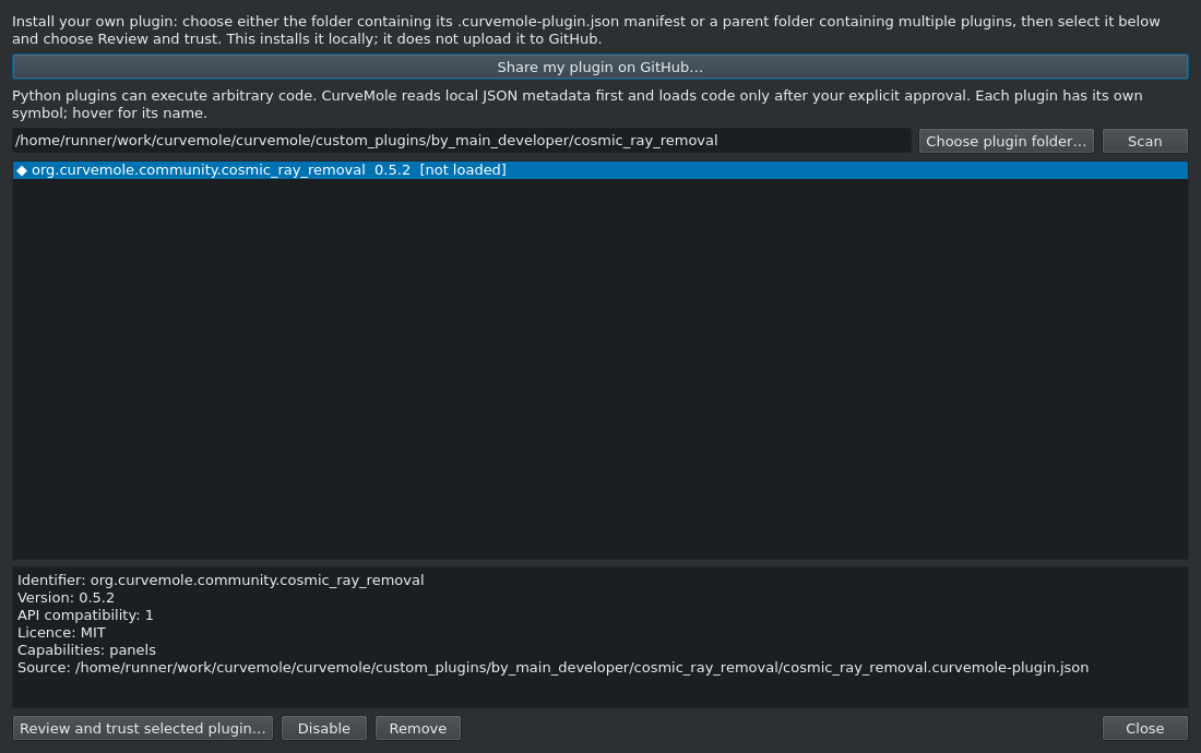
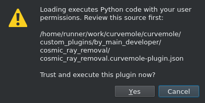
- Select the plugin and click Review and trust selected plugin…. Inspect its source and metadata; approve the Trust Python plugin dialog only after deciding to trust this code. Close the manager.
- The plugin panel opens after loading. To reopen it, use View → Plugins: Panels → Cosmic-ray removal: review and clean (the entry also carries its plugin symbol).
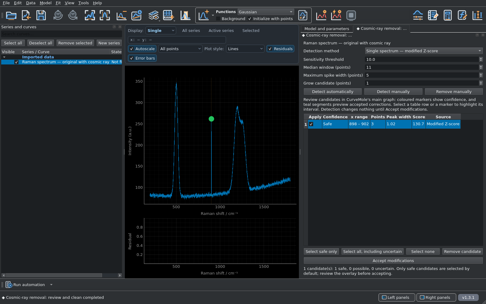
- Keep Single spectrum — modified Z-score with the default threshold 10, median window 11 points, maximum spike width 5 points and candidate growth 1 point. Click Detect automatically.
- Inspect the candidate table and preview. In this example one candidate at approximately 898–902 cm−1 is marked Safe and selected for application. Detection and preview have not changed the stored data.
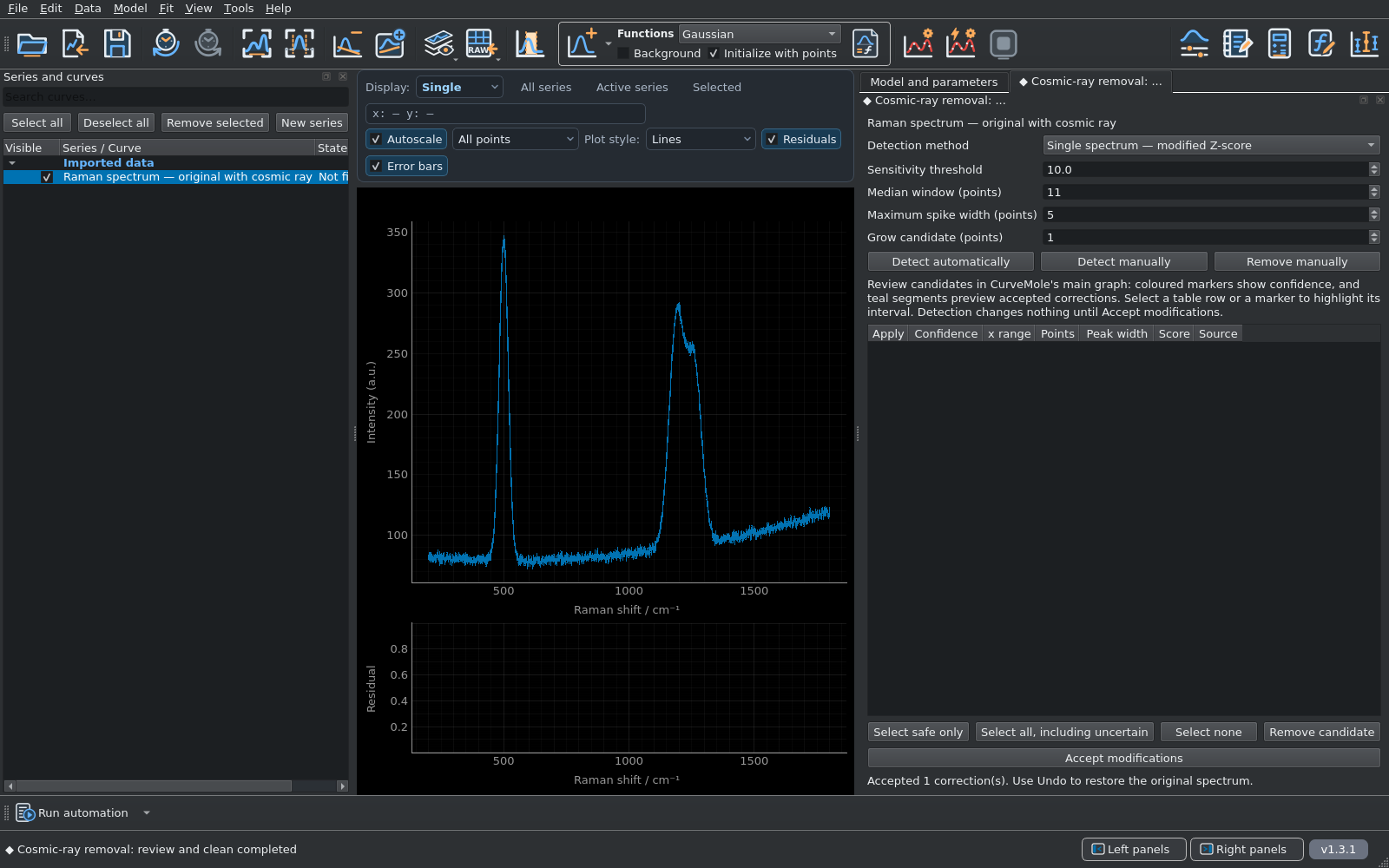
- Check that the selected event is the injected spike, then click Accept modifications. The selected three points are replaced by PCHIP interpolation; the original observations remain available and Undo reverses the correction.
Masking and correction are different choices. The main tutorial keeps measured values and excludes an interval from fitting. The plugin exercise replaces selected values by an estimate. If you analyse the corrected copy, repeat background estimation, fitting and uncertainty analysis on that copy.
Now repeat the analysis with your own data.
You have imported uncertainties, excluded an artefact, constructed and subtracted a background, fitted overlapping bands, examined parameter correlation and saved both numerical results and a complete project.
About the simulation, uncertainty and screenshot versions
The generator uses NumPy seed 1729, area-normalised Gaussian bands and independent Gaussian noise with σy = 2. The polynomial is estimated from three noisy, peak-free observations and then held fixed. Its estimation uncertainty is not included in the subsequent band intervals. The masked artefact is an added one-sample spike; it is not experimental evidence.
The screenshots are captures of the actual CurveMole GUI, generated while executing this workflow. Their capture record identifies the stable software source and numerical results. The website build refreshes the images with the selected stable application version rather than reusing illustrations from an older release.
The capture manifest records the version used for this screenshot set.